In this case, we use as error the square of the horizontal distance, and it is somewhat perturbing that this similarly reasonable approach leads to a best fit that differs from the one obtained when employing vertical distances.
The situation can be made even worse if neither x nor y is a predictor variable. In this case, we want to minimize the shortest distance to a line y = mx + b rather than the vertical (or horizontal) distance. The resulting equations will not be linear, nor can they be made linear. However, Maple will be able to find the critical points with no trouble. There will always be at least two (there may be a third with a huge slope and intercept)- one is the minimum, and the other is a saddle point. It is worth thinking for a few minutes about the geometric interpretation of the saddle point in terms of the problem at hand.
In practice, the perturbing fact that different but reasonable error functions lead to best fits that are different is resolved by knowing what part of the data is the input and what part is predicted from it. This happens often enough, though not always. We thus can make a good choice for E and solve a minimization problem. That settled, we are still left with the problem of demonstrating why our choice for E is a good one.
It is rather easy to write down the solution to the problem in §3: if
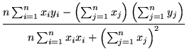 =
=  ,
, If yi are assumed to be the values of random variables Yi which depend linearly upon the xi,
This conclusion follows by merely making assumptions about the inner
products of the data points
(x1,..., xn) and
(y1,..., yn). Staticians often would like to answer questions such
as the degree of accuracy of the estimated value of m and b. For that
one would have to assume more about the probability distribution of the
error variables Yi. A typical situation is to assume that the
![]() above are normally distrubuted, with mean 0 and
variance
above are normally distrubuted, with mean 0 and
variance ![]() . Under these assumptions, the values of m and
b given above are the so-called maximum likelihood estimators for
these two parameters, and there is yet one such estimator for the variance
. Under these assumptions, the values of m and
b given above are the so-called maximum likelihood estimators for
these two parameters, and there is yet one such estimator for the variance
![]() . But, since we assumed more, we can also say more. The estimators
. But, since we assumed more, we can also say more. The estimators
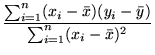
![]() and
and ![]() are normally distributed and, for example, the
mean of
are normally distributed and, for example, the
mean of ![]() is m and its variance is
is m and its variance is
![]() /
/![]() (xi -
(xi - ![]() )2. With this knowledge, one may embark into determining the
confidence we could have on our estimated value for the parameters. We do
not do so in here, but want to plant the idea in the interested reader,
whom we refer to books on the subject.
)2. With this knowledge, one may embark into determining the
confidence we could have on our estimated value for the parameters. We do
not do so in here, but want to plant the idea in the interested reader,
whom we refer to books on the subject.