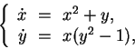
next up previous
Next: About this document ...

Math 331, Fall 2004: Problems Set 6, Due Oct 25


  1. Have Maple find analytic solutions to the following system of differential equations,

    \begin{displaymath}
\left\{
\begin{array}{rcl}
y''(t) - z(t) &\!=\!& e^t, \\
z'(t) - y(t) &\!=\!& 0,
\end{array} \right.
\end{displaymath}

    with initial conditions: $y(0)=1,\ y'(0)=0,\ z(0)=k$. Let us denote the solutions by $y_k(t),\ z_k(t)$ (since they depend on the parameter $k$).

    For $k$ taking all integer values from -10 to 10, and $t \in
[-4,2]$, plot the functions $y_k$ in blue, and the functions $z_k$ in red, all on the same graph. (Yes, you will then have 42 functions plotted on the same graph.) 
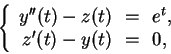
[This is certainly a case when you don't want to retype the functions that Maple finds. You will almost certainly need to read the help page for dsolve. I also found subs, unapply, and seq useful.]

  2. For the functions $y_k(t)$ and $z_k(t)$ found in the previous problem plot the parametric curves $\varphi_k(t) = [y_k(t), z_k(t)]$ for integer values of $k$ between $-5$ and $5$ and $-6 < t <4$ on the same graph. Use the view option of plot to only show what lies in the region $-10<y<10,
-10<z<10$, and use a sequence of colors so that each solution is a different color. [ HINT: you might find something like seq(COLOR(HUE,i/11),i=0..10) useful for the latter.]

  3. Consider the differential equation $\dot{\mathbf {z}}(t) = \mathbf {F}(\mathbf {z}(t))$, where the vector $\mathbf {z}(t)
=(x(t),y(t))$ and the field $\mathbf {F}(x,y) = (-y,x-y)$. Plot a few solutions. What happens to them when $t \to +\infty$? Give a ``Maple-proof'' that this is a general fact for every solution. [A ``Maple-proof'' is an argument that is rigorous once we accept Maple results as incontrovertibly true.]

  4. For the system of differential equations of problem set 5,

    \begin{displaymath}
\left\{
\begin{array}{rcl}
\dot{x} &\!=\!& x^2 + y, \\
\dot{y} &\!=\!& x (y^2 - 1),
\end{array} \right.
\end{displaymath}

    find the eigenvalues and eigenvectors of the Jacobian at the fixed points.

  5. Consider the equations of the glider with no drag term ($R=0$). Use dsolve, type=numeric to solve them numerically with initial conditions $\theta(0)=0$, $v(0)=0.8$. Then solve exactly the linearized system around the fixed point $(\theta_0,v_0) = (0,1)$, with the same initial conditions. Graph the two functions for $0 \le t \le 5$, and give a good estimate of their maximum difference. What happens if we take a larger $t$-range?


next up previous
Next: About this document ...
Moira Chas 2004-10-19